
In part one a neuron was a weighted sum plus a bend, and four small programs showed how a network learns, why it needs the bend, and how it fails outside its data. This part is about the kind of network behind almost every “upload a photo” feature: face unlock, document scanning, defect detection on a production line, the OCR step in your invoice pipeline.
Same rules as before: five small programs, run on a laptop-class machine with no GPU, and the output under each is real. You can run them free in Google Colab.
1. A picture is a grid of numbers, and a filter is a question
To a computer, a grayscale image is a table: one number per pixel, 0 for paper and 1 (or 255) for full ink. A colour image is three such tables, red, green and blue.
The plain network from part one takes that table, flattens it into one long row and feeds every pixel to every neuron. That works, but it throws away the one thing that matters most in a picture: which pixels are next to which. Pixel 57 and pixel 58 could be on opposite sides of the image, as far as that network knows.
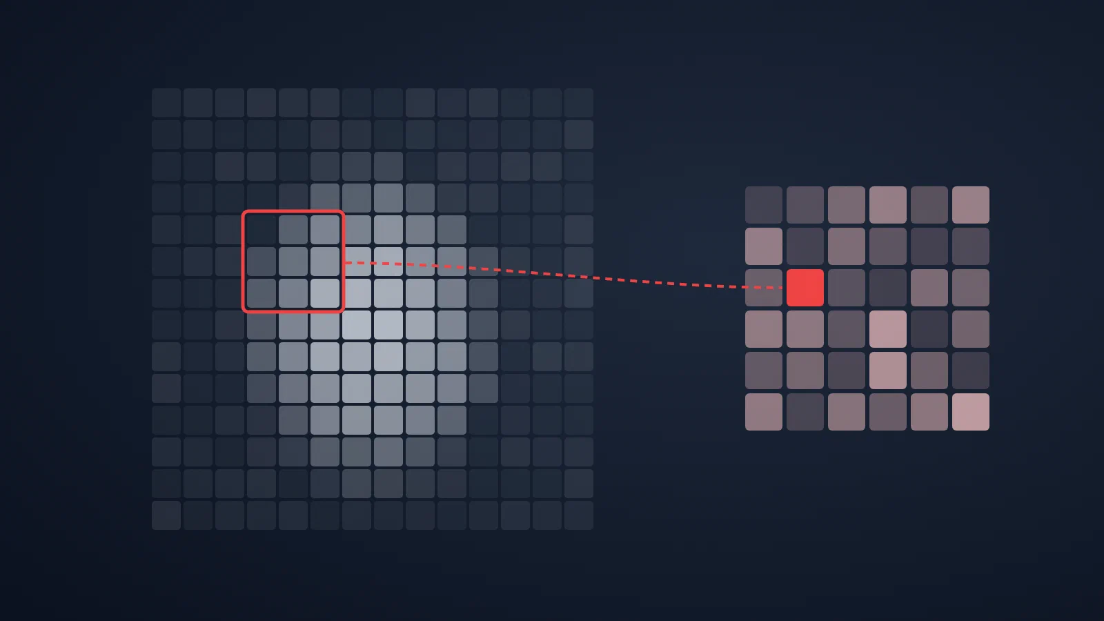
A convolution keeps the neighbours together. Take a small grid of weights, the filter, typically 3×3. Put it on the top-left corner of the image, multiply each pixel by the weight on top of it, add up, and write the result down. Slide one pixel right and repeat, row by row, until the whole image is covered.
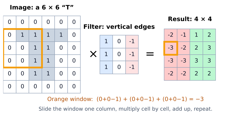
In code, with a 6×6 picture of a “T” and two hand-made filters:
import numpy as np

# A 6x6 picture of a "T": 1 = ink, 0 = paper
img = np.array([
    [0, 0, 0, 0, 0, 0],
    [0, 1, 1, 1, 1, 0],
    [0, 0, 1, 1, 0, 0],
    [0, 0, 1, 1, 0, 0],
    [0, 0, 1, 1, 0, 0],
    [0, 0, 0, 0, 0, 0],
])

vertical_edges = np.array([[1, 0, -1],
                           [1, 0, -1],
                           [1, 0, -1]])
horizontal_edges = vertical_edges.T

def convolve(image, kernel):
    kh, kw = kernel.shape
    out = np.zeros((image.shape[0] - kh + 1, image.shape[1] - kw + 1), dtype=int)
    for r in range(out.shape[0]):
        for c in range(out.shape[1]):
            window = image[r:r + kh, c:c + kw]      # a 3x3 piece of the picture
            out[r, c] = np.sum(window * kernel)     # multiply cell by cell, add up
    return out

print("vertical edges:\n", convolve(img, vertical_edges))
print("horizontal edges:\n", convolve(img, horizontal_edges))
vertical edges:
 [[-2 -1  1  2]
 [-3 -2  2  3]
 [-3 -3  3  3]
 [-2 -2  2  2]]
horizontal edges:
 [[-1 -2 -2 -1]
 [ 1  1  1  1]
 [ 0  0  0  0]
 [ 1  2  2  1]]
Read the output as answers. The vertical-edge filter asks “is there ink on one side of me and paper on the other?” The strongest answers are in the outer columns, where the sides of the stem are, and the sign tells you which side. The horizontal-edge filter is exactly zero in the third row, the middle of the stem, where nothing changes from top to bottom.
Two details make this cheap. The filter is small, so it has only 9 weights. And it is the same 9 weights at every position, so a filter that learned to spot an edge spots it anywhere in the picture. A convolutional layer is just many such filters, 32 or 64 of them, each producing its own map of answers.
What it means for you: in a real network nobody writes these filters. They are weights, and training finds them, exactly like the weights in part one. You will see what they learned in program 4.
2. Max pooling: keep the strongest answer, drop the rest
After a convolution, networks usually pool: cut the map into 2×2 blocks and keep only the largest number from each.
import numpy as np

feature_map = np.array([
    [1, 3, 0, 2],
    [4, 2, 1, 0],
    [0, 1, 5, 6],
    [2, 0, 7, 1],
])
# split into 2x2 blocks and keep the largest value of each
pooled = feature_map.reshape(2, 2, 2, 2).max(axis=(1, 3))
print(pooled)
[[4 2]
 [2 7]]
Sixteen numbers become four. Pooling has no weights and learns nothing; it keeps “there was a strong edge somewhere around here” and forgets exactly where. Every pooling step quarters the data the next layer has to process.
What it means for you: pooling is what keeps the work shrinking layer after layer; without it, every layer would process a full-size image. It also buys a little tolerance to small movements, though, as program 5 shows, much less than people assume.
3. Same size, better eyes
Now a real data set. Fashion-MNIST has 70,000 small grayscale photos of clothes in ten classes, 60,000 for training and 10,000 for testing, published by Zalando’s research team as a harder stand-in for the classic handwritten digits.[2]
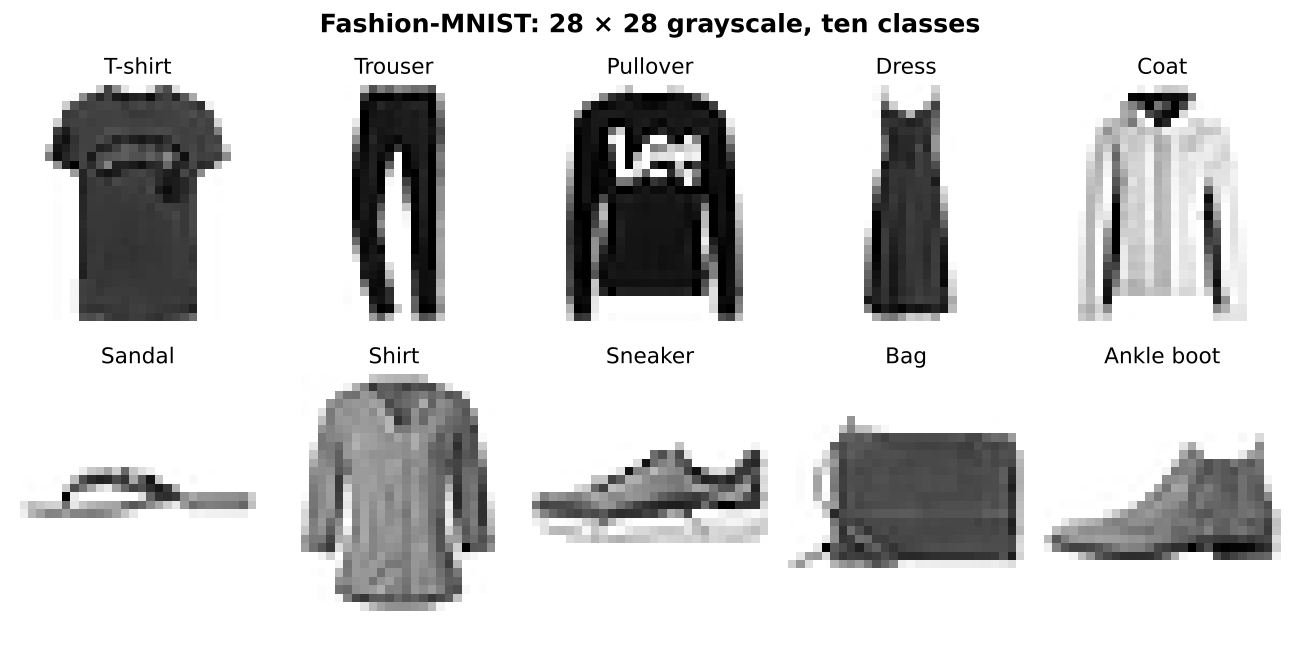
I trained two models on it, five passes over the data each. The first is the plain network from part one. The second is a small convolutional neural network (CNN): two rounds of convolution and pooling in front of a smaller dense layer. That shape goes back to Yann LeCun’s work on reading cheques in the 1990s.[1]
import time
import numpy as np
import keras

(x_train, y_train), (x_test, y_test) = keras.datasets.fashion_mnist.load_data()
x_train, x_test = x_train / 255.0, x_test / 255.0           # pixels 0..255 -> 0..1
x_train, x_test = x_train[..., None], x_test[..., None]     # add the channel: 28x28x1

def dense():
    return keras.Sequential([
        keras.Input(shape=(28, 28, 1)),
        keras.layers.Flatten(),                              # 784 numbers in a row
        keras.layers.Dense(128, activation="relu"),
        keras.layers.Dense(10, activation="softmax"),        # one probability per class
    ])

def cnn():
    return keras.Sequential([
        keras.Input(shape=(28, 28, 1)),
        keras.layers.Conv2D(32, (3, 3), activation="relu"),  # 32 learned 3x3 filters
        keras.layers.MaxPooling2D((2, 2)),
        keras.layers.Conv2D(64, (3, 3), activation="relu"),  # 64 filters on top of those
        keras.layers.MaxPooling2D((2, 2)),
        keras.layers.Flatten(),
        keras.layers.Dense(64, activation="relu"),
        keras.layers.Dense(10, activation="softmax"),
    ])

for name, build in [("dense", dense), ("cnn", cnn)]:
    keras.utils.set_random_seed(42)
    model = build()
    model.compile(optimizer="adam", loss="sparse_categorical_crossentropy", metrics=["accuracy"])
    t0 = time.time()
    model.fit(x_train, y_train, epochs=5, verbose=0)
    train_s = time.time() - t0
    loss, acc = model.evaluate(x_test, y_test, verbose=0)
    t0 = time.time()
    model.predict(x_test, verbose=0)
    ms = (time.time() - t0) / len(x_test) * 1000
    model.save(f"{name}.keras")
    print(f"{name:5}  params {model.count_params():7,}  train {train_s:4.0f} s  "
          f"test accuracy {acc:.2%}  predict {ms:.3f} ms/image")
dense  params 101,770  train   22 s  test accuracy 86.77%  predict 0.071 ms/image
cnn    params 121,930  train   87 s  test accuracy 89.99%  predict 0.096 ms/image
Three points of accuracy sounds small. Count the mistakes instead: 1,323 wrong out of 10,000 for the plain network, 1,001 for the CNN. A quarter fewer errors, with almost the same number of parameters.
Now look at where those parameters are. The two convolutional layers together hold 18,816 weights (320 + 18,496). The dense layer after them holds 102,464. The filters that do the “seeing” are cheap, because each one is 9 weights reused at every position. Yet the CNN took four times longer to train, because every filter weight is used once per position: 676 times per image in the first layer, 121 times in the second.
What it means for you: two different numbers size two different things. Parameters size memory: the model file, the RAM, the GPU you need to load it (part one). How often each parameter is used sizes compute: training time, inference latency, the cost per thousand images. Ask a vendor for both.
4. Look inside: what the filters learned
Nobody told the network to look for edges. Here is one ankle boot from the test set and what seven of the 32 learned filters in the first layer made of it, bright where the filter’s answer is strong:
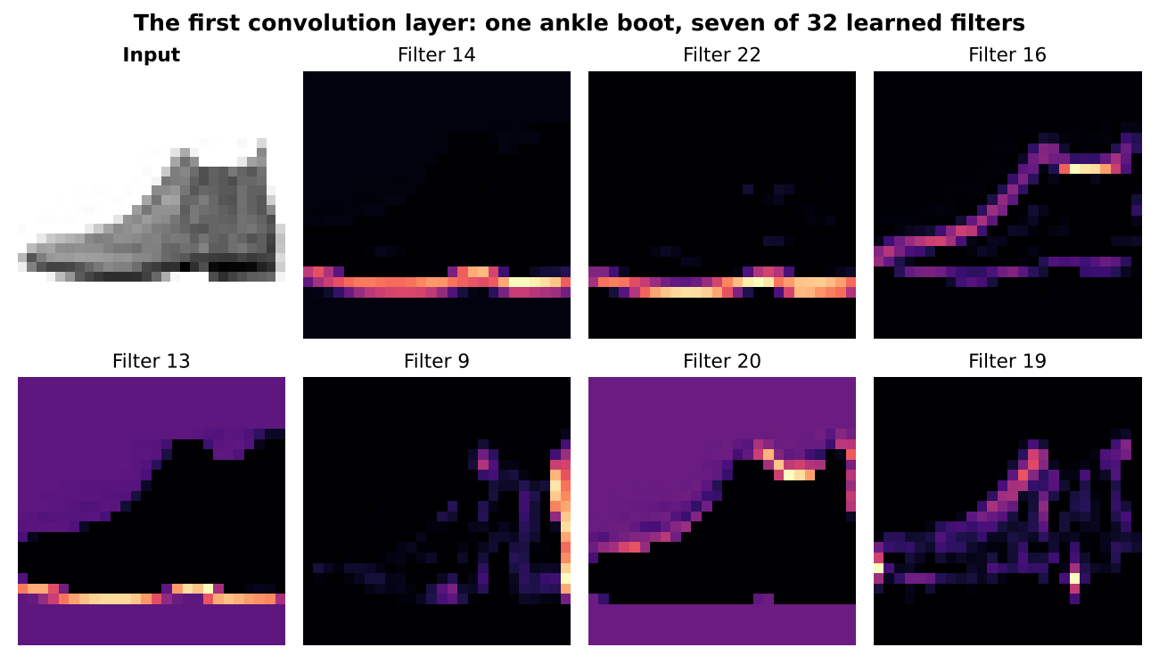
Training found, on its own, filters for the sole, for the upper outline, for the back of the heel, and for “this is background”. The next layer combines these into larger parts, and the dense layer at the end turns parts into “ankle boot”.
The same model also tells you where it struggles. Accuracy per class on the test set, weakest first:
names = ["T-shirt", "Trouser", "Pullover", "Dress", "Coat",
         "Sandal", "Shirt", "Sneaker", "Bag", "Ankle boot"]
dense, cnn = keras.models.load_model("dense.keras"), keras.models.load_model("cnn.keras")

pred = cnn.predict(x_test, verbose=0).argmax(axis=1)
for c in np.argsort([np.mean(pred[y_test == c] == c) for c in range(10)]):
    mask = y_test == c
    wrong = np.bincount(pred[mask][pred[mask] != c], minlength=10)
    print(f"{names[c]:10} {np.mean(pred[mask] == c):6.1%}   most often mistaken for: {names[wrong.argmax()]}")
Shirt       60.2%   most often mistaken for: Coat
T-shirt     82.7%   most often mistaken for: Shirt
Pullover    87.7%   most often mistaken for: Coat
Coat        91.8%   most often mistaken for: Pullover
Dress       92.2%   most often mistaken for: Coat
Ankle boot  94.6%   most often mistaken for: Sneaker
Bag         96.3%   most often mistaken for: Pullover
Sandal      98.1%   most often mistaken for: Sneaker
Sneaker     98.1%   most often mistaken for: Ankle boot
Trouser     98.2%   most often mistaken for: Dress
A “90% model” gets trousers right 98% of the time and shirts only 60%. At 28×28 pixels a shirt, a coat and a pullover are honestly hard to tell apart.
What it means for you: never accept a single accuracy figure for a model that will make decisions. Ask for accuracy per class, or per document type, per product line, per customer segment. The average hides exactly the cases that will reach your support desk.
5. The shift test
Fashion-MNIST photos are all neatly centred. What happens if I move every test image 4 pixels to the right, the kind of offset a slightly different camera or a sloppy crop produces?
shifted = np.zeros_like(x_test)
shifted[:, :, 4:, :] = x_test[:, :, :-4, :]
for name, m in [("dense", dense), ("cnn", cnn)]:
    a = m.evaluate(x_test, y_test, verbose=0)[1]
    b = m.evaluate(shifted, y_test, verbose=0)[1]
    print(f"{name:5}  as trained {a:.2%}   shifted 4 px {b:.2%}")
dense  as trained 86.77%   shifted 4 px 24.50%
cnn    as trained 89.99%   shifted 4 px 36.23%
Both collapse. The CNN holds up a little better, but from 90% to 36% is not “robust”. This surprises people, because the textbook story is that convolution and pooling make CNNs indifferent to where things are. Researchers have measured the same gap in large, modern image models.[3] The filters do work everywhere, but everything after them was trained on centred clothes only.
The fix is not a smarter layer. It is better data: show the model shifted images while it trains. Keras can do that on the fly with one extra layer, which moves every training image by a random amount and does nothing when the model is used for predictions:
keras.layers.RandomTranslation(0.15, 0.15, fill_mode="constant"), # training only: move each image up to ~4 px
Same CNN, same five passes, with that layer added in front:
cnn + shifted training as trained 87.70% shifted 4 px 85.59%
On shifted images it goes from 36% to 86%. On the original centred images it loses two points in five passes, because each image is now a moving target. Here is one boot, as each model saw it:
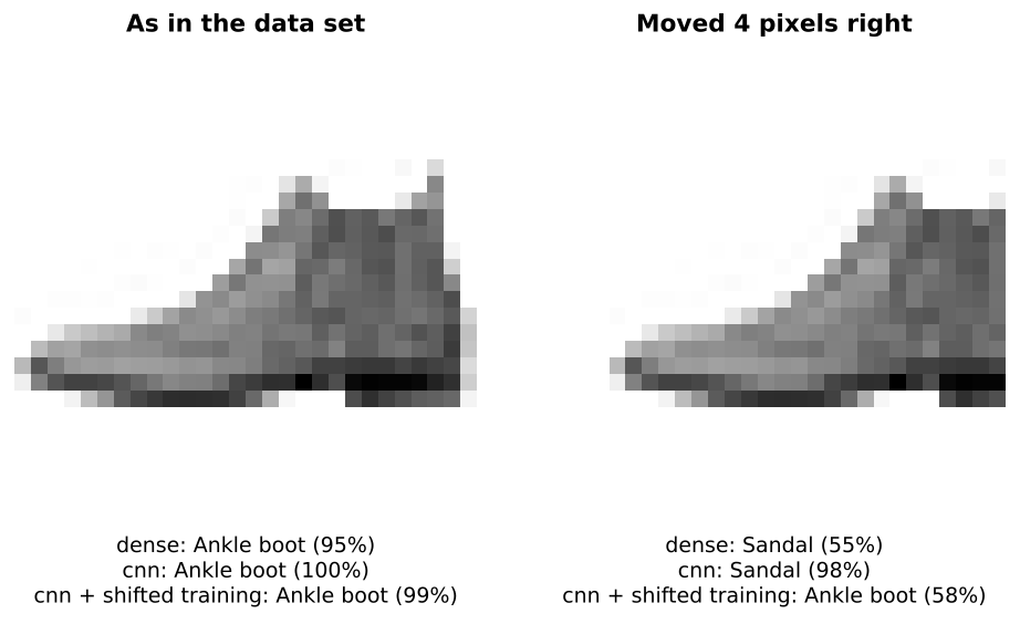
Look at the CNN’s answer for the moved boot: Sandal, 98%. Confidence is not correctness.
What it means for you: this is part one’s lesson again, with pictures. A vision model knows the camera, the lighting, the crop and the angle of its training data, and nothing else. Before go-live, test it with your own images taken the way your users will take them, not with the vendor’s demo set. If the production camera changes, re-test.
The short version
- A convolution slides a small filter over the image and asks the same question everywhere. Training writes the filters.
- Pooling keeps the strongest answer in each block. It shrinks the data and forgets exact positions.
- CNNs see better for the same size, here a quarter fewer mistakes, but they cost more compute per image.
- Ask for accuracy per class. A 90% model can be a 60% model on the case you care about.
- Test with your own images. A 4-pixel shift took a 90% model to 36%. Training on shifted images brought it back to 86%.
Everything above ran on a 2-vCPU Linux machine without a GPU, with TensorFlow 2.21 and Keras 3.15, in under four minutes of training in total. Training times vary by a few seconds between runs; with the fixed seed, the accuracies repeat exactly.
References
- LeCun, Y., Bottou, L., Bengio, Y. and Haffner, P. (1998). Gradient-based learning applied to document recognition. Proceedings of the IEEE, 86(11), 2278–2324. doi.org
- Xiao, H., Rasul, K. and Vollgraf, R. (2017). Fashion-MNIST: a Novel Image Dataset for Benchmarking Machine Learning Algorithms. arXiv:1708.07747. arxiv.org
- Azulay, A. and Weiss, Y. (2019). Why do deep convolutional networks generalize so poorly to small image transformations? Journal of Machine Learning Research, 20(184), 1–25. arxiv.org


Comments
Comments are stored in GitHub Discussions. Sign in with GitHub to comment or react.