
Every AI service you put in an architecture diagram, whether it is a chat model, an OCR API or a fraud score, is built from one very small idea, repeated a very large number of times. You do not need the maths to design around it, but you do need to know what that idea is, because it explains the things that end up on your bill and in your incident reports.
So instead of a lecture, here are four small programs. I ran each one, and the output under each is real. You can run them yourself for free in Google Colab or on any laptop with Python, NumPy and Keras.
1. One neuron is three lines of arithmetic
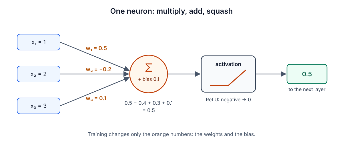
The idea is old. Warren McCulloch and Walter Pitts described an artificial neuron in 1943, modelled loosely on a brain cell that fires when its inputs are strong enough.[1] The modern version does three things:
- It multiplies each input by a weight.
- It adds them up, plus one extra number called the bias.
- It passes the result through an activation function, which bends it. The most common one, ReLU, turns anything negative into zero.
In code:
import numpy as np

def neuron(x, w, b):
    z = np.dot(w, x) + b          # weighted sum of the inputs, plus a bias
    return max(0.0, z)            # activation: ReLU, negative becomes 0

print(neuron(np.array([1.0, 2.0, 3.0]), np.array([0.5, -0.2, 0.1]), 0.1))
print(neuron(np.array([1.0, 2.0, 3.0]), np.array([-0.5, -0.2, 0.1]), 0.1))
0.5
0.0
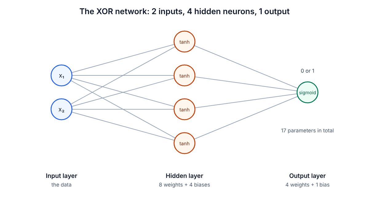
Same inputs, one weight flipped, and the neuron goes quiet. That is the whole unit. A network is many of these in layers: an input layer that receives the data, one or more hidden layers in the middle, and an output layer that gives the answer. Each neuron passes its output to every neuron in the next layer. “Deep learning” just means many hidden layers.
What it means for you: a trained model is nothing but its weights and biases. Together they are called parameters, and a model file is a long list of them. Everything about running a model follows from how many there are.
2. Training is guess, measure, nudge
Nobody sets the weights by hand. You give the network examples and let it adjust. Here I hide a rule, y = 2x − 1, in six data points and let a single neuron (one weight, one bias, no activation) find it:
import numpy as np

x = np.array([-1.0, 0.0, 1.0, 2.0, 3.0, 4.0])
y = 2 * x - 1                       # the rule we hide in the data

w, b = 0.3, 0.0                     # 1. start with a guess
lr = 0.05                           # how big a nudge each step takes

for step in range(501):
    pred = w * x + b                # 2. predict
    err = pred - y
    loss = np.mean(err ** 2)        #    and measure how wrong (mean squared error)
    if step in (0, 10, 50, 100, 500):
        print(f"step {step:3}  loss {loss:9.6f}  w {w:6.3f}  b {b:6.3f}")
    dw = 2 * np.mean(err * x)       # 3. which way should w and b move to cut the error?
    db = 2 * np.mean(err)
    w -= lr * dw                    # 4. nudge them that way
    b -= lr * db

print(f"x = 3.5  ->  {w * 3.5 + b:.4f}   (the rule says 6)")
step   0  loss 10.831667  w  0.300  b  0.000
step  10  loss  0.388339  w  1.733  b -0.175
step  50  loss  0.005596  w  1.968  b -0.901
step 100  loss  0.000028  w  1.998  b -0.993
step 500  loss  0.000000  w  2.000  b -1.000
x = 3.5  ->  6.0000   (the rule says 6)
It never saw the rule, only the examples, and it found w = 2, b = −1. Step 3 is the only clever part. Working out which way to move every weight in a network with many layers is called backpropagation. Paul Werbos described it in 1974,[3]
and Rumelhart, Hinton and Williams made it famous in 1986.[4]
Moving a small step in that direction, over and over, is gradient descent. Large models train the same way, with billions of weights instead of two.
With a library, the same network takes four lines. This is Keras 3, the API that ships with TensorFlow:
import keras

keras.utils.set_random_seed(42)
model = keras.Sequential([keras.Input(shape=(1,)), keras.layers.Dense(1)])
model.compile(optimizer="sgd", loss="mean_squared_error")
model.fit(x, y, epochs=500, verbose=0)
print(model.predict(np.array([[3.5]]), verbose=0))
[[5.999189]]
Note the answer: 5.999189, not 6. The model learned an approximation, not the rule.
What it means for you: a model’s output is a very good estimate, never a guarantee. Anything downstream that needs an exact answer, such as an amount, an ID or a yes/no that triggers a payment, needs a check, a threshold or a human after the model.
3. The bend is what makes it smart
Why the activation function? Without it, every neuron is a weighted sum, and a weighted sum of weighted sums is still a weighted sum. Stack as many layers as you like: the network can only draw straight lines.
The classic test is XOR: output 1 when exactly one of two inputs is 1. No straight line separates those cases. In 1969 Minsky and Papert showed that a single-layer network cannot learn it,[2]
and the result helped push neural networks out of fashion for over a decade. Here is the same small network trained twice, once with straight-line hidden neurons and once with tanh, which bends:
x = np.array([[0, 0], [0, 1], [1, 0], [1, 1]], dtype=float)
y = np.array([0, 1, 1, 0], dtype=float)          # XOR: 1 when exactly one input is 1

def train(hidden_activation):
    keras.utils.set_random_seed(7)
    model = keras.Sequential([
        keras.Input(shape=(2,)),
        keras.layers.Dense(4, activation=hidden_activation),   # hidden layer
        keras.layers.Dense(1, activation="sigmoid"),           # output: 0..1
    ])
    model.compile(optimizer=keras.optimizers.Adam(0.05), loss="binary_crossentropy")
    model.fit(x, y, epochs=500, verbose=0)
    return model.predict(x, verbose=0).ravel().round(2)

print("linear hidden layer:", train(None))
print("tanh hidden layer:  ", train("tanh"))
linear hidden layer: [0.5 0.5 0.5 0.5]
tanh hidden layer:   [0. 1. 1. 0.]
Without the bend, the network gives up and answers 0.5, “no idea”, for every case. With it, all four answers are right. The sigmoid on the output squeezes the result between 0 and 1, so it reads as a probability.
What it means for you: the vendor’s choice of layers and activations is the model. You never tune it when you call an API, but it is why two models with the same number of parameters can behave very differently on your data.
4. Outside its data, a model is confidently wrong
The last program teaches a deeper network y = x², but only with values of x between −2 and 2. Then I ask it about 1.5, 3 and 10:
keras.utils.set_random_seed(1)
x = np.linspace(-2, 2, 200).reshape(-1, 1)
y = x ** 2                                   # trained only on -2..2

model = keras.Sequential([
    keras.Input(shape=(1,)),
    keras.layers.Dense(16, activation="tanh"),
    keras.layers.Dense(16, activation="tanh"),
    keras.layers.Dense(1),
])
model.compile(optimizer=keras.optimizers.Adam(0.01), loss="mean_squared_error")
model.fit(x, y, epochs=300, verbose=0)

for v in (1.5, 3.0, 10.0):
    print(f"x = {v:4}  model {model.predict(np.array([[v]]), verbose=0)[0,0]:7.2f}   true {v*v:6.2f}")
x =  1.5  model    2.24   true   2.25
x =  3.0  model    5.60   true   9.00
x = 10.0  model    6.12   true 100.00
Inside the range it trained on, it is almost perfect. Just outside, it is off by a third. Far outside, it answers 6.12 when the truth is 100. Look at how it fails: no error and no warning, just a number that looks exactly as trustworthy as the good ones.
What it means for you: this is the most important of the four. A model trained on last year’s transactions, one country’s documents or one factory’s sensors will give you answers outside that range without blinking. Monitor what goes in, not only what comes out. If the inputs drift away from the training data, expect the quality to drop before anyone reports it.
The one multiplication that sizes your infrastructure
Back to the y = 2x − 1 model. Keras reports its size:
Trainable params: 2 (8.00 B)
Two parameters, 4 bytes each. That multiplication, parameters × bytes per parameter, is the first number to work out for any model you plan to host:
| Model | Parameters | Weights at 16-bit (2 bytes) |
|---|---|---|
| The line above | 2 | 4 bytes |
| The XOR network | 17 | 34 bytes |
| A 7-billion-parameter language model | 7,000,000,000 | 14 GB |
| A 70-billion-parameter language model | 70,000,000,000 | 140 GB |
That is only the weights, and only for inference, the forward pass that answers a request. The GPU also needs memory for each request in flight. Training needs far more: with the usual mixed-precision setup and the Adam optimizer, the model state alone takes about 16 bytes per parameter, because the GPU must also hold gradients and optimizer statistics.[5] A 7B model goes from 14 GB to serve to over 100 GB to train, before any training data.
This is why most teams call a hosted model or fine-tune a small one instead of training from scratch, and why “can we run it ourselves?” is first a question about GPU memory, not about code.
The short version
- A neuron multiplies, adds and bends. A model is its parameters, saved as a file of numbers.
- Training is guess, measure, nudge, repeated billions of times. It is expensive. Running the result is far cheaper.
- Outputs are estimates. Put validation after the model wherever exactness matters.
- Models fail quietly outside their data. Monitor inputs for drift.
- Size is parameters × bytes. Do that multiplication before you pick a GPU, a SKU or a vendor.
References
- McCulloch, W. S. and Pitts, W. (1943). A logical calculus of the ideas immanent in nervous activity. Bulletin of Mathematical Biophysics, 5, 115–133. link.springer.com
- Minsky, M. and Papert, S. (1969). Perceptrons: An Introduction to Computational Geometry. MIT Press.
- Werbos, P. J. (1974). Beyond Regression: New Tools for Prediction and Analysis in the Behavioral Sciences. PhD thesis, Harvard University.
- Rumelhart, D. E., Hinton, G. E. and Williams, R. J. (1986). Learning representations by back-propagating errors. Nature, 323, 533–536. nature.com
- Rajbhandari, S., Rasley, J., Ruwase, O. and He, Y. (2019). ZeRO: Memory Optimizations Toward Training Trillion Parameter Models. arXiv:1910.02054. arxiv.org



Comments
Comments are stored in GitHub Discussions. Sign in with GitHub to comment or react.